ITMIX Experiment 2016

Note 1: this post was originally published in March 2016 on the OGGM website. It is now reproduced here with a few small modifications.

Note 2: in the meantime, the ITMIX group discussed the preliminary results at the EGU assembly in Vienna. It turns out that OGGM is doing quite a good job! More about this by the end of 2016.

Note 3: the paper summarizing the experiment is online for review! Visit this link to read and discuss the manuscript.

OGGM participates to the ITMIX experiment organised by the IACS Working Group on Glacier Ice Thickness Estimation.

The idea is to compare several models able to provide a distributed estimate of glacier ice thickness. The participants can submit their estimations for one (or more) of 18 selected glaciers. The first phase of the experiment is supposed to be “blind”, i.e. the participants are not aware of the actual thickness of the glaciers they are modelling.

The deadline for the experiment was February 29th. Definitely too early for OGGM, with which we had performed the inversion for the European Alps only. We still didn’t want to miss this opportunity and started an intense development phase to make OGGM applicable globally. After quite a lot of work we are now able to provide an estimate for all glaciers (except for Starbuck in Antarctica). While this surely marks an important step in the development of OGGM, this project raised many questions and digged a few issues out, since (as you will see below), nothing is easy when doing global scale distributed modelling.

ITMIX preprocessing

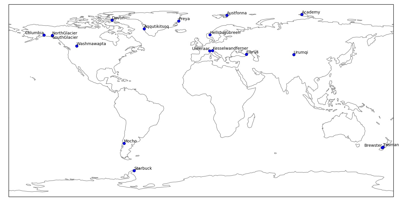
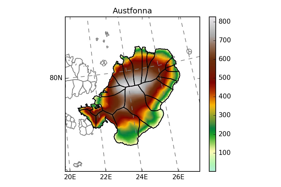
The glaciers chosen by the ITMIX organisors are heterogeneous: valley glaciers, ice-caps, marine-terminating…

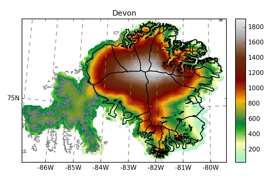
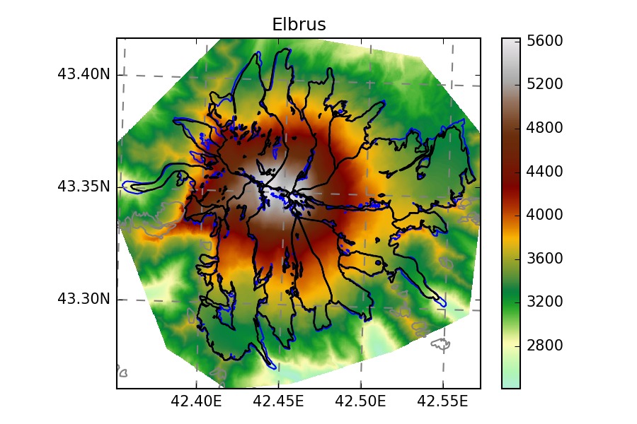
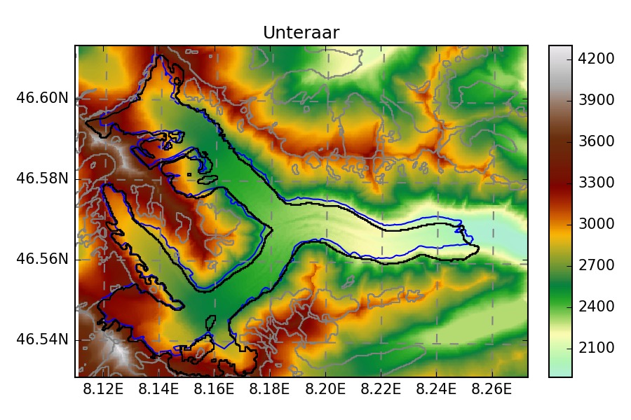
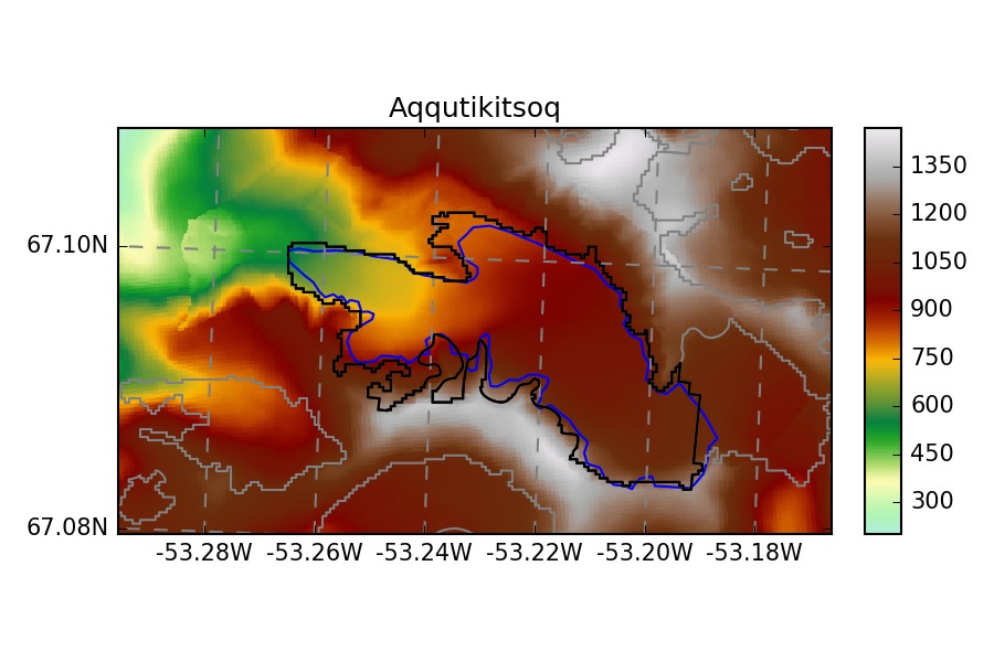
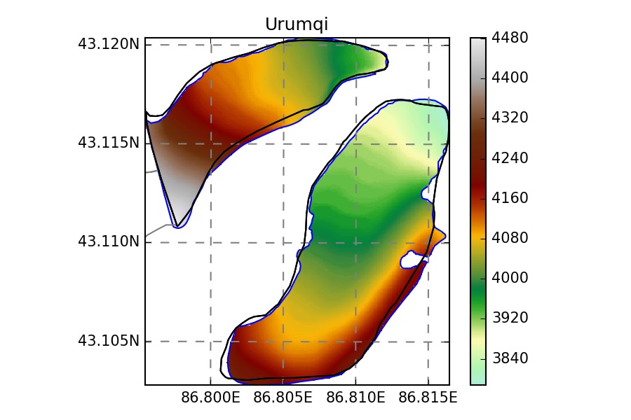Blue outlines: ITMIX , Black outlines: RGI. Note that some ITMIX glaciers have no topography outside of their outlines.

The first thing we needed to do is to formalize all this data so that OGGM can deal with it. This turned out to be a bit complicated since the ITMIX data was not standardized:

• we updated the RGI outlines with the ITMIX ones where possible
• for ice-caps, we kept the RGI outlines because OGGM currently needs the “pieces of cake” to compute the centerlines
• we decided to to compute the inversion on the OGGM local grids, not on the IMIX maps. This is important because OGGM makes decisions about the grid spacing it uses. Furthermore, the entire workflow is depending on these standardized local maps. We introduced a new routine in the pipeline in order to update the SRTM/ASTER topography with the ITMIX one. This also was not trivial because some ITMIX topographies are stopping directly at the glacier boundary

OGGM preprocessing

Topography

OGGM uses following DEM data:

• SRTM V4.1 for [60S, 60N] (http://srtm.csi.cgiar.org/)
• GIMP DEM for Greenland (https://bpcrc.osu.edu/gdg/data/gimpdem)
• Corrected DEMs for Svalbard, Iceland, and North Canada (http://viewfinderpanoramas.org/dem3.html)
• ASTER V2 elsewhere

The corrected DEMs where necessary because ASTER data has many issues over glaciers. Take for example the DEM for two glaciers in Iceland:

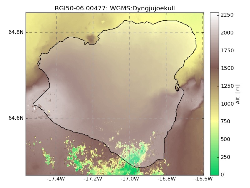
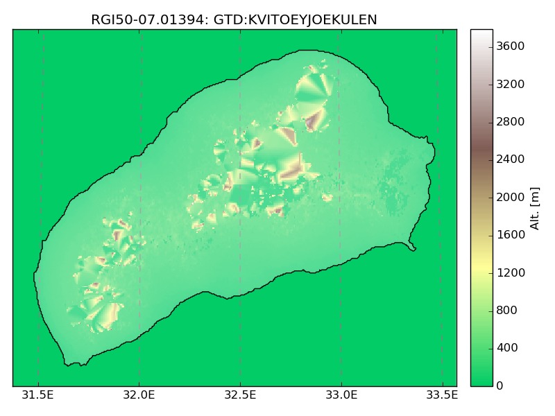
Note that the hypsometry provided in RGI V5 (M. Huss) also contains these errors. While the problems with the right plot are obvious, the topography of the glacier on the left (Dyngjujoekull) is practically impossible to detect (and therefore correct) automatically. On the plot below, I show the hypsometry that OGGM computed and the one by RGI:

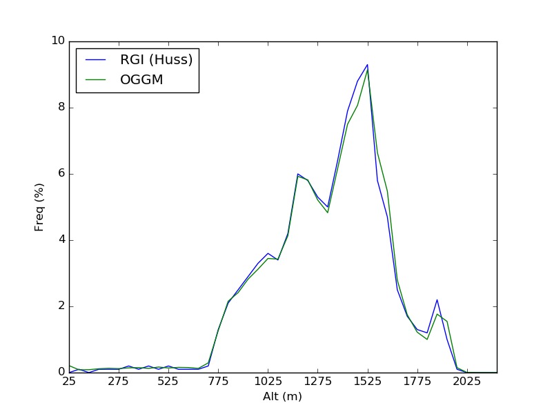
Up to a few discrepancies due to projection issues, we both have the problem of non-zero bins below 750 m a.s.l. Fortunately, thanks to the dem3 data these problems are now resolved in OGGM:

There is potential for even better coverage of corrected DEM (there is an ongoing PR about that).

Calibration data

Another obstacle to global coverage was that the databases required for calibration (WGMS FoG and GlaThiDa) are not “linked” to RGI, i.e. there is no way to know which RGI entity corresponds to each database entry. Thanks to the work of Johannes Landmann at UIBK we now have comprehensive links with global coverage.

Some of the ITMIX glaciers were in the database, I removed them manually for the sake of the experiment (“blind run”):

• WGMS: Kesselwandferner, Brewster, Devon, Elbrus, Freya, Hellstugubreen, Urumqi
• GlaThiDa: Kesselwandferner, Unteraar

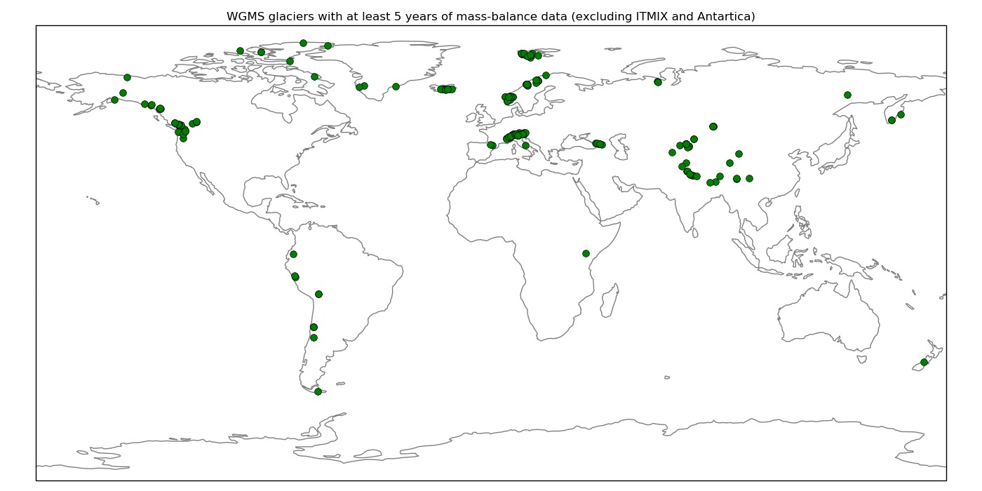
These leaves us with 196 WGMS glaciers with at least 5 years of mass-balance data available for calibration of the mass-balance:

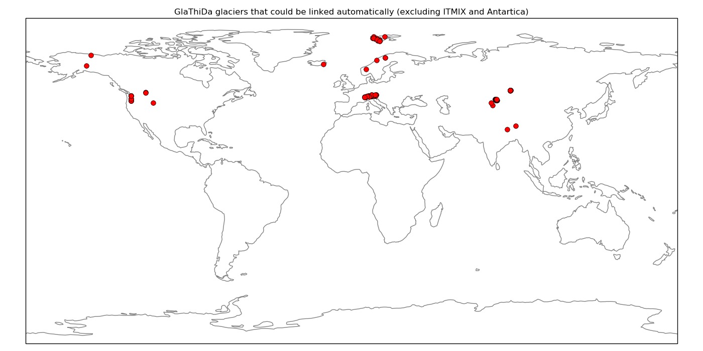
And 133 GlaThiDa glaciers with glacier-wide average thickness estimates. The coverage of GlaThiDa is not very good, which is probably a problem:

Inversion procedure

Refer to the general documentation for details about the inversion procedure.

Here we go directly to the calibration results of the ice-thickness inversion. OGGM currently has only one free parameter to tune for the ice thickness inversion: Glen’s creep parameter A. This is very similar to Farinotti et al., (2009)¹, with the difference that we are not calibrating A for each glacier individually: we tried to do that, but didn’t manage (yet).

Land-terminating glaciers

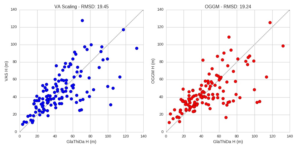
Currently, A is varied until the glacier-wide thickness computed by OGGM minimizes the RMSD with GlaThiDa. We removed all ice-caps and marine-terminating glaciers from the dataset in order to avoid these specific cases (135 glaciers left). Here are the results of the calibration (left: volume-area scaling, right: OGGM):

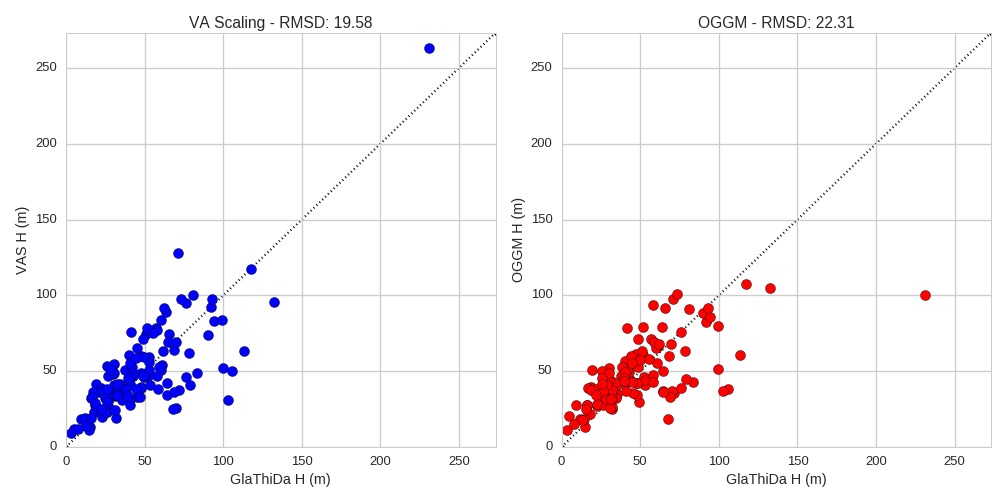
We can see that OGGM has a slightly lower score than volume-area scaling (VAS). This is due to the presence of a couple of outliers. In particular, the thickest glacier in GlaThiDa and VAS is strikingly thin in OGGM: this is the Black Rapids glacier in Canada, which is quite well mentioned in the literature because it is a surging glacier. Closer inspection in OGGM reveals that this glacier has one of the lowest mass-balance gradient. CRU precipitation is 849 mm yr^-1 (after application of the 2.5 correction factor!), which I assume is too low.

We recall here that one central difference between our approach and that of Huss and Farinotti (2012)² is that we use real climate data to compute the apparent mass-balance, and thus have glacier specific mass-balance gradients. This is a strength but can also become a burden. The mass-balance gradient depends mostly on precipitation, but also on temperature and its seasonal cycle. Here I show the apparent mass-balance gradient in the ablation area of all GlaThiDa glaciers:

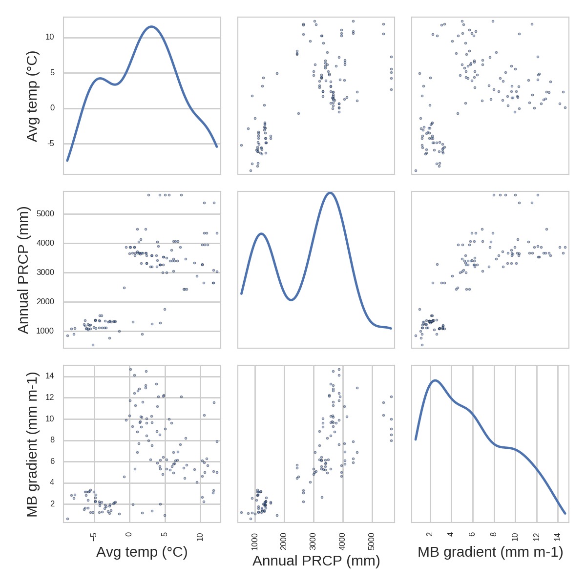
Is the MB gradient related to the error OGGM makes in comparison to GlaThiDa?

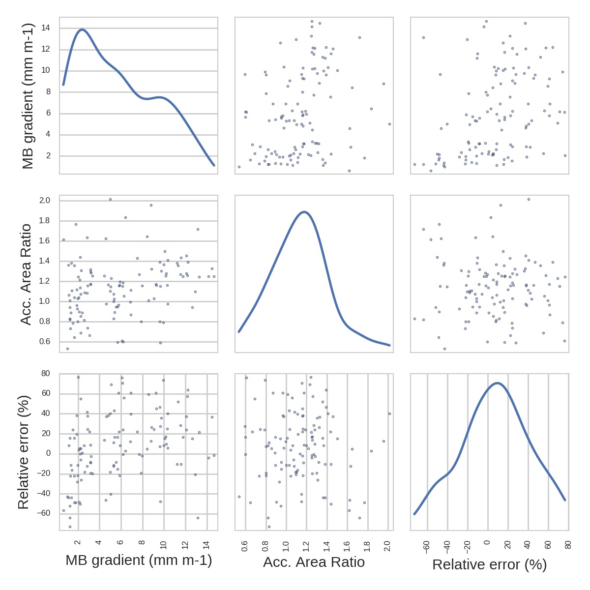
No, not really. And this is similar with all other glacier characteristics I could look at until now. The error that OGGM makes is not easily attributable to specific causes… It it would, that would be great! Indeed, this would allow maybe to define a rule for the calibration factor A. If you have ideas at which parameter to look at, let me know!

VAS vs OGGM

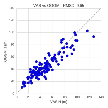
I don’t want the calibration to be too altered by the Black Rapids outlier, so I removed it from the calibration set. The plot now looks better, and after this little hack OGGM is even slightly better than VAS:

What is really interesting however is that OGGM and VAS are incredibly similar in their dissimilarity with GlaThiDa. So similar that if we plot the two approaches together on a scatter, one could argue that the thousands of lines of code of OGGM really aren’t worth the effort ;). I think that I have to talk to David Bahr about this, he will surely be pleased.

A problem with large glaciers?

These results for the reference glaciers availble in GlaThiDa were somehow OK, but the issue with the Black Rapids glacier made me wonder a little bit and I decided to have a closer look. In the figure below I compare the OGGM inversion results with VAS for all glaciers I have at hand for the experiment (ITMIX + WGMS + GlaThiDa, land-terminating, no ice-caps).

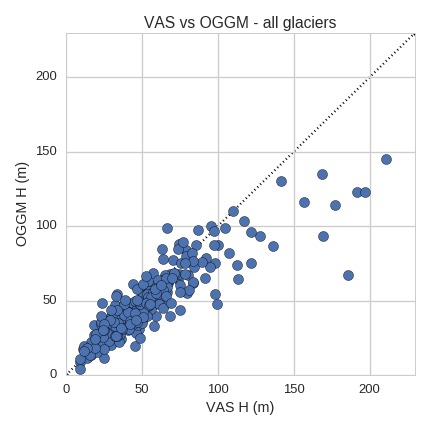
After many hours (days?) of searching for a reasonable explanation for this behavior, I had to renounce. [Edit: a master student is now working on this topic!]

An ice-caps?

This one is easier: ice caps are cut into smaller pieces of cake, instead of being considered as a large glacier. Like VAS, OGGM will also fail since the volume of glaciers is expected to grow with a power law to its area. The flowline methodology followed by OGGM on ice caps is very likely to underestimate the total ice volume.

Marine-terminating glaciers

Using the apparent mass-balance method for calving glaciers will lead to overestimated thicknesses. In the future, OGGM will intend to parametrize mass-flux at calving fronts. For ITMIX, we will consider mass loss by calving for Columbia glacier only. From Rasmussen et al., (2011)³, we assume two possible calving rates for Columbia: 4.3 and 8.0 km³ ice eq a^-1, to which we arbitrarily add a third case with 12 km³ ice eq a^-1. This mass loss at the calving front is distributed over the glacier and added to the apparent mass-balance, resulting in total ice volumes of 250, 273, and 291 km³, respectively.

Putting all this together

We find an optimised factor for A of 3.22 (i.e. our A is three times larger than the standard of 2.4 10^-24 described by Cuffey and Paterson (2010)⁴. This makes sense since we do not consider the sliding velocity in the inversion, which means that we need an ice which is less stiff to compensate.

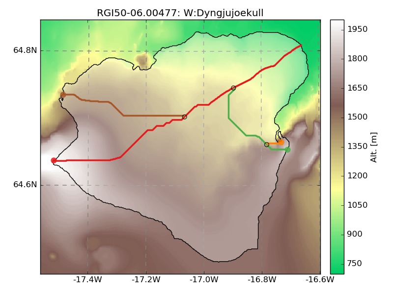
The inversion procedure in OGGM is not designed to provide a distributed estimate of glacier thickness: in particular, the glacier widths in OGGM are not always geometrical as in Farinotti et al. (2009): they are also corrected so that the altitude-area distribution of the glacier is preserved.

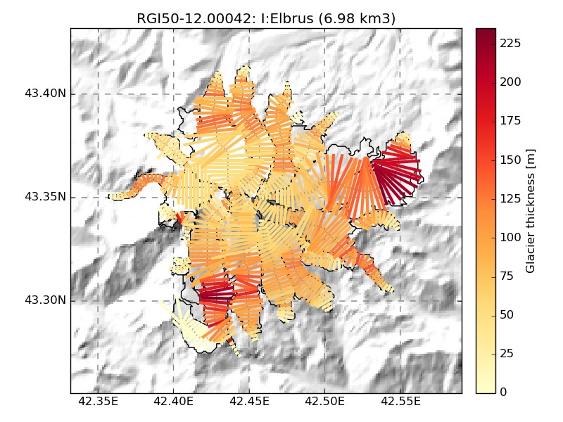
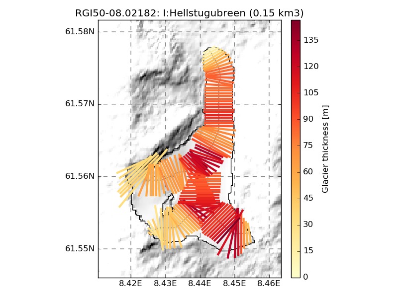
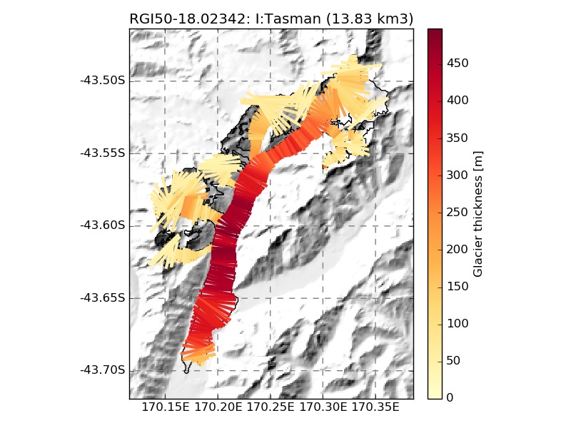
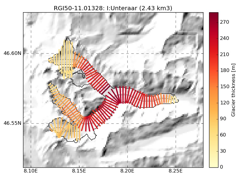
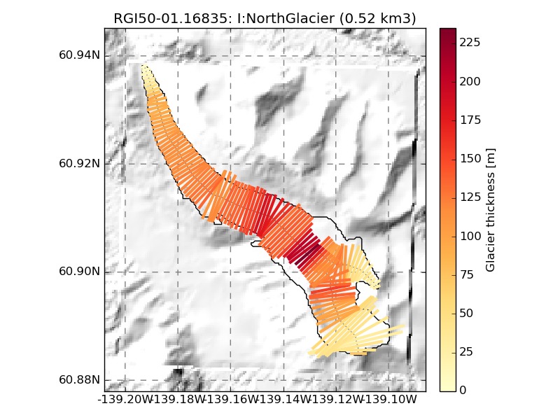
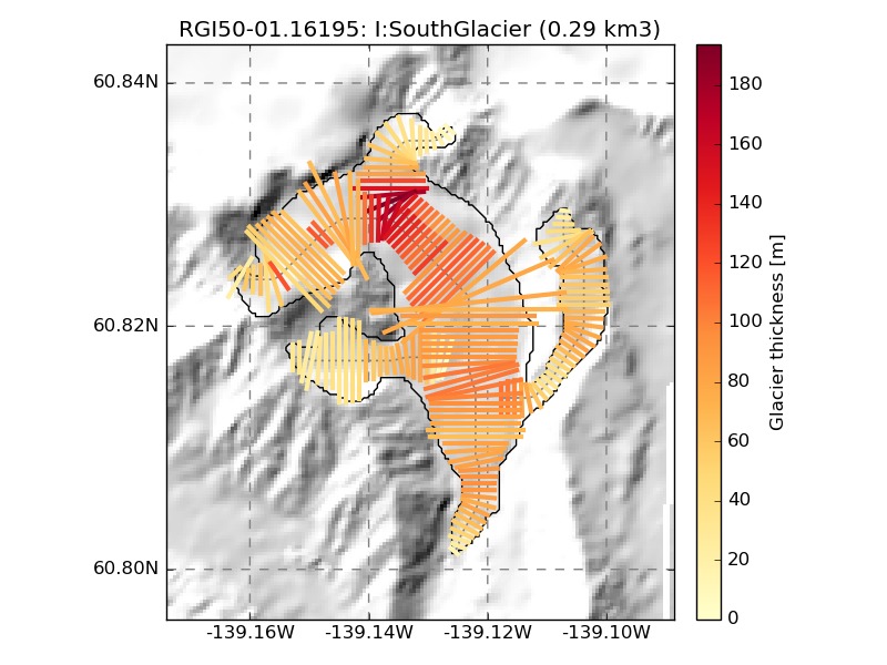
We show a few examples of the inversion procedure in OGGM, which is meant to provide the input to a flowline model:

Distributed ice thickness

In a final step, we had to somehow interpolate the flowline thicknesses to the ITMIX map. Here again we made the choice to keep as much logic as possible within the standard OGGM framework and defined a new task, distribute_thickness. We compute the ice thickness on the OGGM local map and simply interpolate our results on the high resolution ITMIX grid only at the very end.

The distribution works as follows:

• for each pixel, the closest flowlines thicknesses within a 100m altitude range are interpolated using an inverse distance weight
• this value is then corrected with a factor depending on the distance to the glacier outlines
• finally, the thickness is corrected with a factor \(1 / \alpha^{\frac{N}{N+2}}\) as in Farinotti et al. (2009). Since I had no time to check if this correction works better, I submitted two versions of the interpolation (with or without local slope correction).

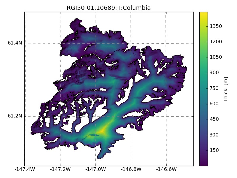
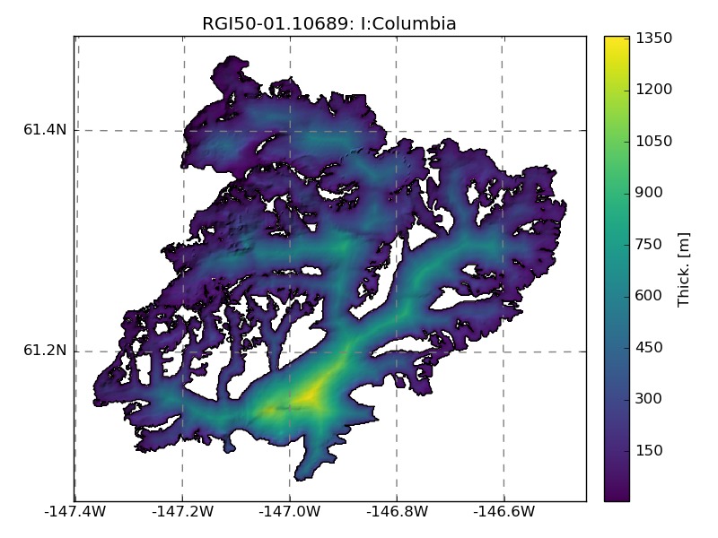
An example of the interpolation for Columbia glacier with (left) or without (right) slope correction:

For the ice caps, the interpolation methods lead to similar results. However, it is very likely that the flowline methodology used by OGGM is not working properly.

Conclusions

We were able to provide an estimate of ice thickness for all glaciers except Starbuck in Antarctica. I am less confident about the distributed maps than the total volume estimates. I am also much less confident about the ice-caps and also less confident about the larger glaciers than the smaller ones.

References

---